Projection Formula Derived from the Definition
Orthogonal projection is defined by two conditions: the projected vector lies in the chosen direction or subspace, and the leftover vector is perpendicular to that direction or subspace.
Starting from those conditions makes the familiar formulas follow naturally instead of appearing from nowhere.
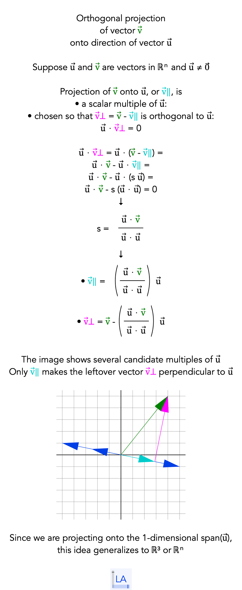
The first diagram derives projection onto the direction of one vector.
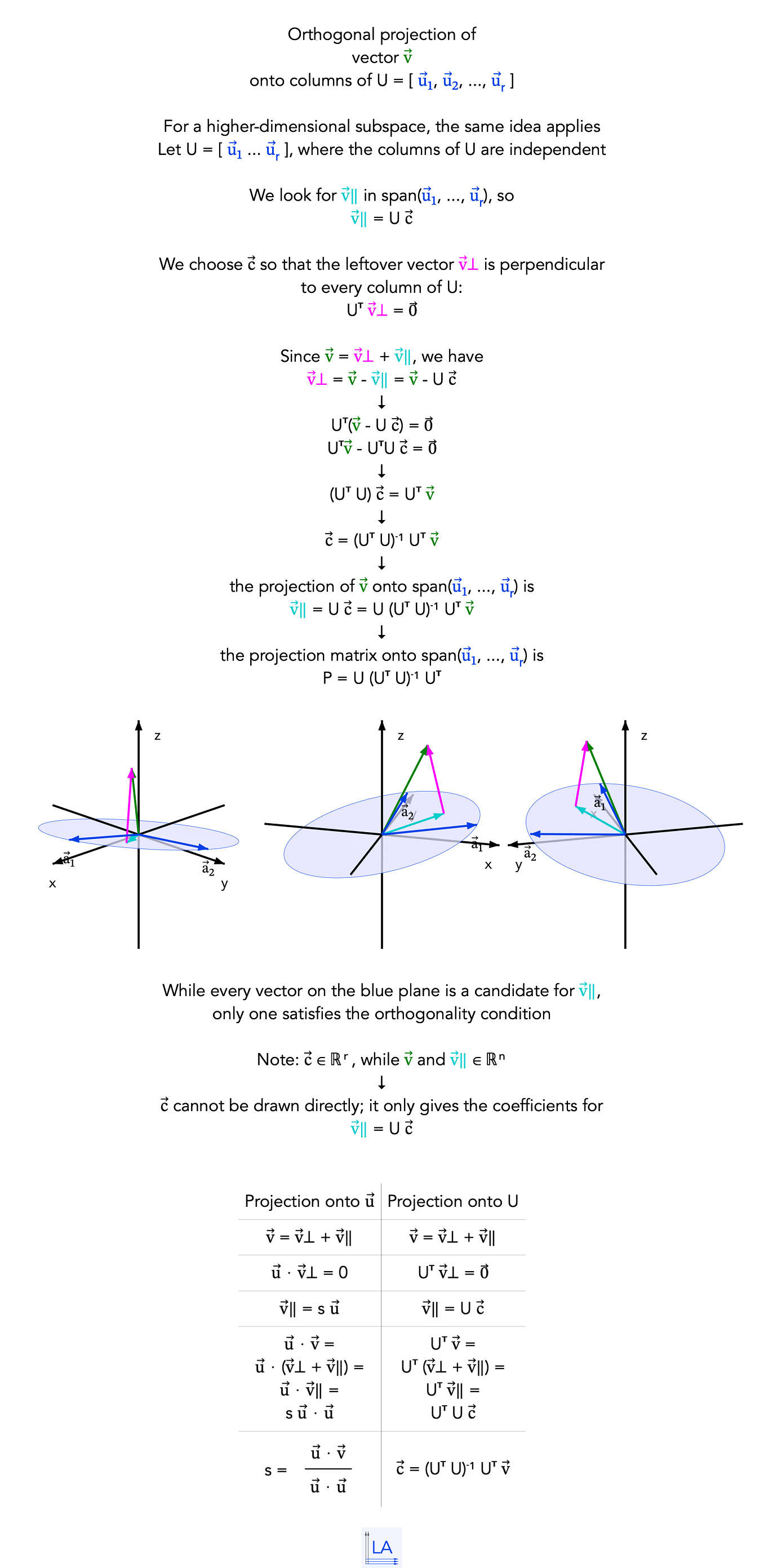
The second uses exactly the same idea for projection onto the column space of a full-column-rank matrix.
Projection onto the direction of one vector
We require the projection v⃗∥ to be a scalar multiple of u⃗, so v⃗∥ = s u⃗.
The defining orthogonality condition u⃗ · (v⃗ − v⃗∥) = 0 determines the scalar s and gives the usual projection formula.
Click the image to open the full-size version.
Projection onto the column space of U
For U = [u⃗₁, u⃗₂, ..., u⃗ᵣ], the projection must have the form v⃗∥ = Uc⃗.
Requiring the residual to be perpendicular to every column of U gives Uᵀ(v⃗ − Uc⃗) = 0⃗, which leads directly to the normal equations and the projection matrix.
Click the image to open the full-size version.
Concept
In both cases, projection is obtained by splitting the vector into
v⃗ = v⃗⊥ + v⃗∥.
The projected part belongs to the chosen subspace, while the residual belongs to its orthogonal complement.
For one direction, the unknown is a scalar s.
For a subspace spanned by several columns, the unknown is a coordinate vector c⃗.
The matrix formula is therefore the direct higher-dimensional version of the one-vector formula.
Structure
Projection onto span(u⃗) uses
v⃗∥ = s u⃗ and u⃗ · v⃗⊥ = 0.
Projection onto col(U) uses
v⃗∥ = Uc⃗ and Uᵀv⃗⊥ = 0⃗.
Solving these parallel conditions gives
s = (u⃗ · v⃗)/(u⃗ · u⃗) in the one-dimensional case and
c⃗ = (UᵀU)−1Uᵀv⃗ in the general full-column-rank case.