Gram-Schmidt Orthogonalization — Stepwise Visualization in 2D and 3D
This page presents Gram-Schmidt orthogonalization as a geometric process rather than as a list of formulas.
The images below show how the columns are gradually corrected and normalized in 2D and 3D, making the construction of an orthonormal basis visible step by step.
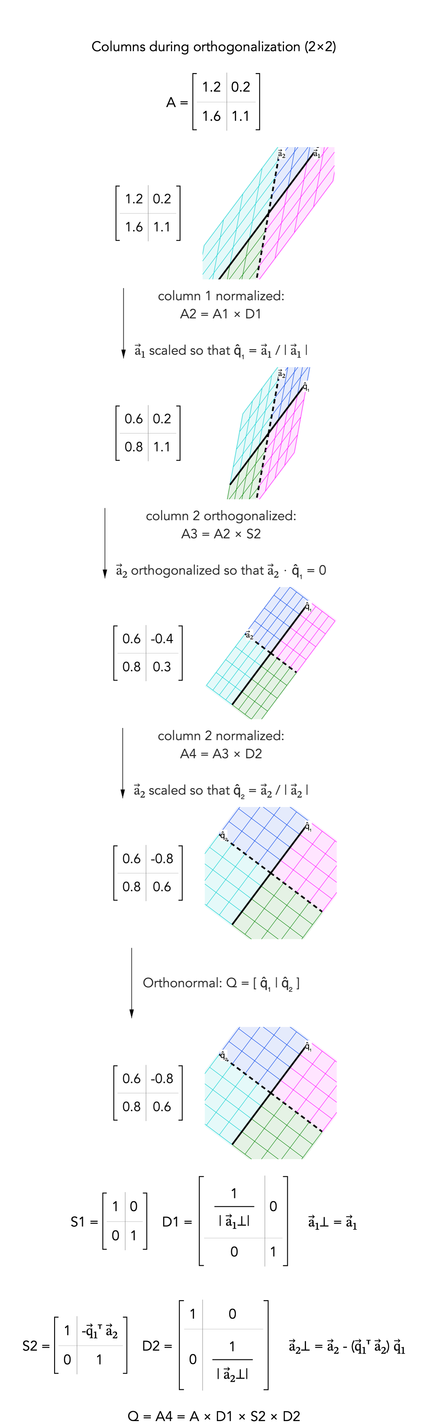
Stepwise orthogonalization in 2D
In two dimensions, the first column is normalized, then the second is orthogonalized against it and normalized.
The static diagram shows the sequence as a chain of intermediate matrices, while the animation shows the same process unfolding continuously.
Click the diagram to open the full-size image.
Animated 2D process
The geometric changes correspond to the symbolic updates that normalize the first column and then remove the component of the second column in that direction.
This makes the construction of the orthonormal basis visible as a continuous motion.
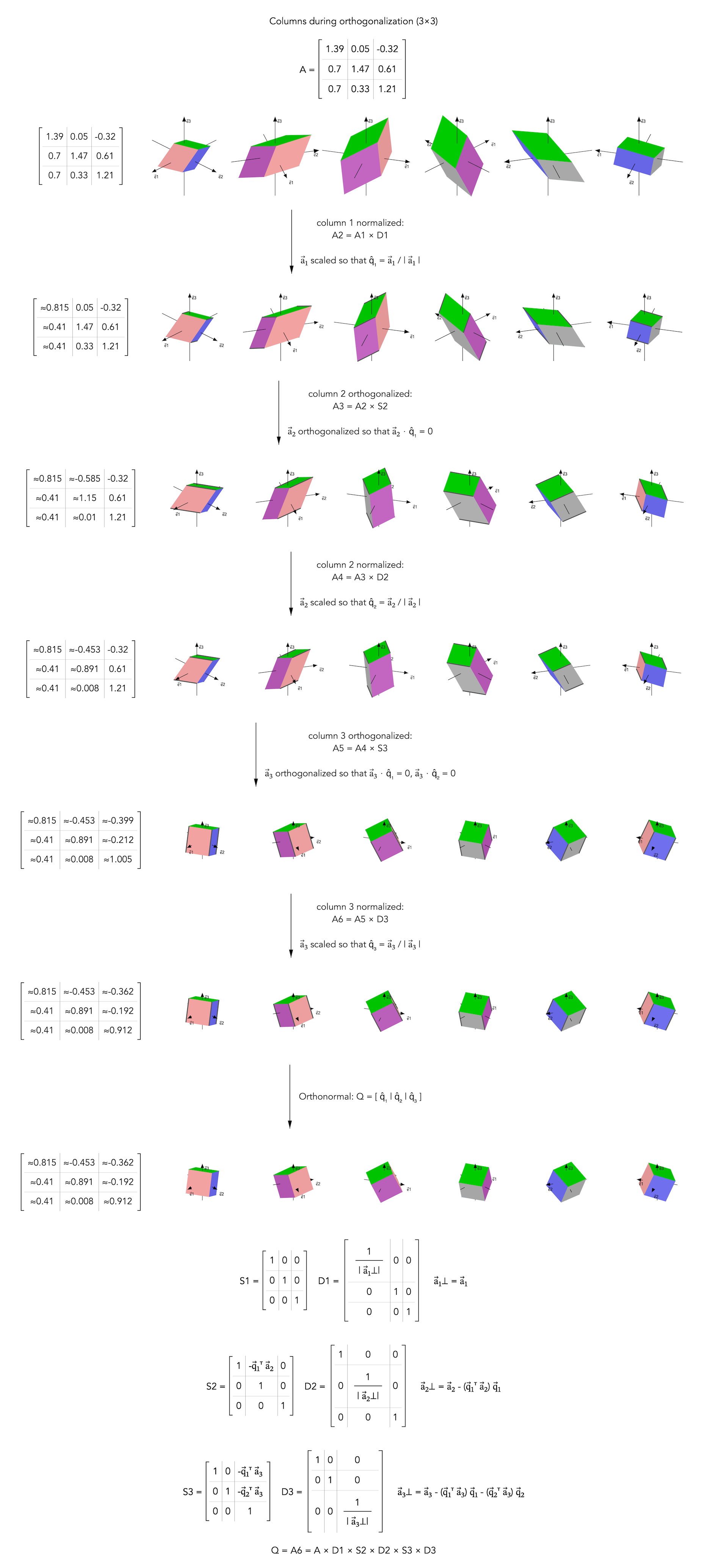
Stepwise orthogonalization in 3D
In three dimensions, the same logic continues one column at a time.
After the first normalization, the second column is made orthogonal to the first, then normalized, and finally the third is corrected against the first two and normalized.
Click the diagram to open the full-size image.
Animated 3D process
Each new direction is corrected against the previously established orthogonal directions, making the construction of the orthonormal basis visible step by step.
This is the process viewpoint behind the factorization.
Gram-Schmidt orthogonalization visualized as semi-transparent cubes (same matrix)
This animation shows the same 3D Gram-Schmidt process with a different visual representation.
Semi-transparent cubes with coordinates in the interval [0, 1] make the motion and final destinations of the vectors easier to visualize.
The semi-transparent version uses the same matrix as the 3D animation above.
It shows the same orthogonalization and normalization process while making the evolving column geometry easier to inspect.
Concept
Gram-Schmidt converts independent columns into orthonormal columns.
In matrix form, this produces the factor Q of QR decomposition, while the coefficients used during the process are recorded in the upper-triangular factor R.
These images emphasize the process viewpoint:
the columns are not replaced all at once, but are corrected and normalized in a definite order, with each step acting on one active column.
One useful way to read the process is as a sequence of right-side updates.
Scale and shear are removed step by step from the original matrix, producing the orthonormal matrix Q, while the removed transformations accumulate into the upper-triangular factor R.