Visual Guide to Diagonalizable 2×2 Matrices
This visual guide compares several common classes of diagonalizable 2×2 matrices,
showing their geometry, eigenvectors and corresponding change-of-basis factorizations side by side.
For each matrix, the direct action of A is compared with the three-step route
A = C D C−1: change to the eigenvector basis, scale independently by the eigenvalues,
and return to the original coordinates.
Geometry, eigenvectors and diagonalization
The chart compares several diagonalizable 2×2 matrices, including scaling, shear-like and symmetric cases.
Each row shows the matrix, the geometric effect on the unit circle or grid, the eigenvector and eigenvalue information,
and the corresponding diagonalization viewpoint. Click the image to open the full-size version.
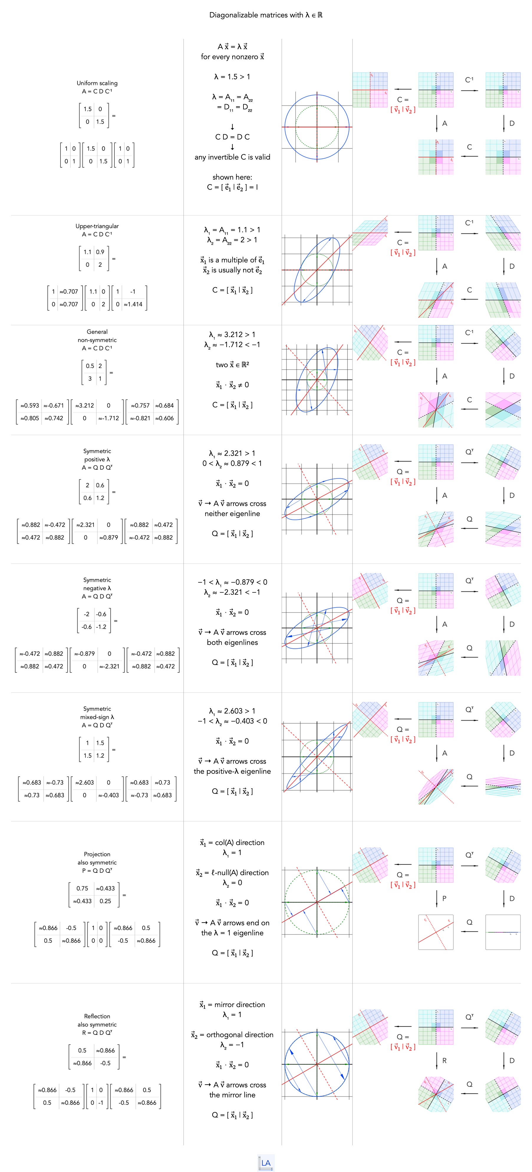
What the diagram shows
A matrix is diagonalizable when it has enough independent eigenvectors to form a basis.
Placing those eigenvectors as the columns of C turns the transformation into
A = C D C−1, where D records the eigenvalue scalings.
Why diagonalization helps
In the eigenvector basis, the transformation no longer mixes coordinate directions.
Each coordinate is scaled independently, so the middle matrix is diagonal.
The visual therefore connects three viewpoints at once: the geometry in the original coordinates,
the eigenvector structure, and the simpler diagonal action seen after a change of basis.