Least Squares as Projection in R³ (3 Observations, 2 Parameters)
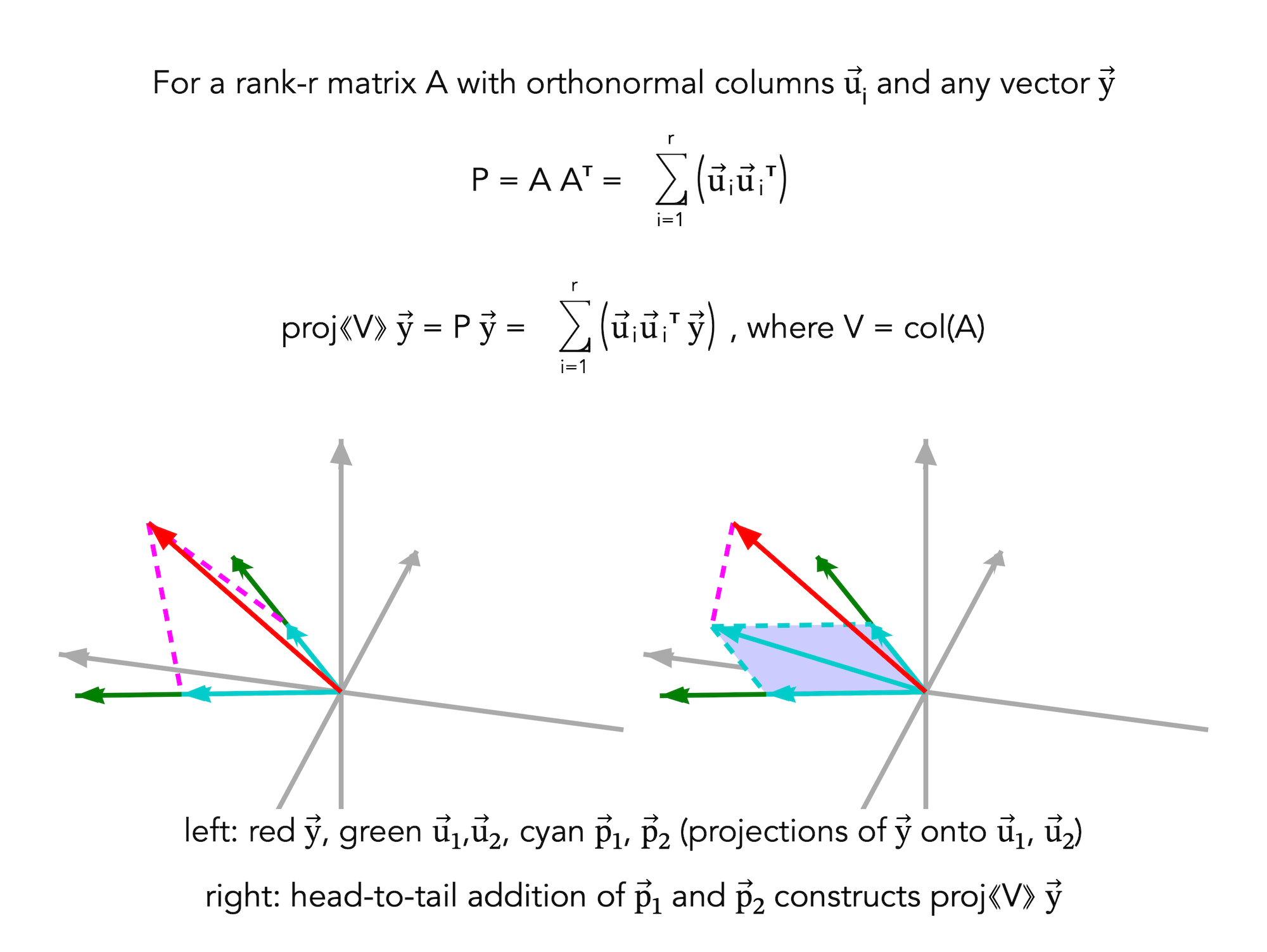
Least squares in this setting means finding the vector ŷ = Xβ̂ in the column space of a 3 × 2 design matrix X that is closest to the data vector y ∈ R³. Geometrically, col(X) is a plane in R³, ŷ is the orthogonal projection of y onto that plane and the residual r = y − ŷ is perpendicular to the plane.
Visual
Model and geometry
With three data values and two parameters, the design matrix has the form X ∈ ℝ3×2, the parameter vector is β ∈ R² and the data vector is y ∈ R³. Every candidate fit has the form Xβ, so all fitted vectors lie in col(X), a subspace of R³ of dimension at most 2.
If the two columns of X are independent, then col(X) is a plane. Least squares chooses the point of that plane that minimizes the Euclidean distance to y.
Key equations
The equation Xᵀ(y − Xβ̂) = 0 states that the residual is orthogonal to every column of X, hence orthogonal to the whole column space.
Why R³ appears here
The ambient space is determined by the number of observations, not by the number of parameters. Three observed values produce a data vector with three coordinates, so y lives in R³. Two parameters produce a two-dimensional model subspace inside that ambient space, which is why the fit can be drawn as projection onto a plane in R³.
Query phrases
- least squares as projection in R3
- three observations two parameters least squares geometry
- orthogonal projection interpretation of least squares
- why residual is perpendicular to column space
- normal equations geometric meaning
Reference
External reference: Wikipedia — Ordinary least squares, Projection section