Powers of a 2D Matrix with Complex Eigenvalues: Concepts

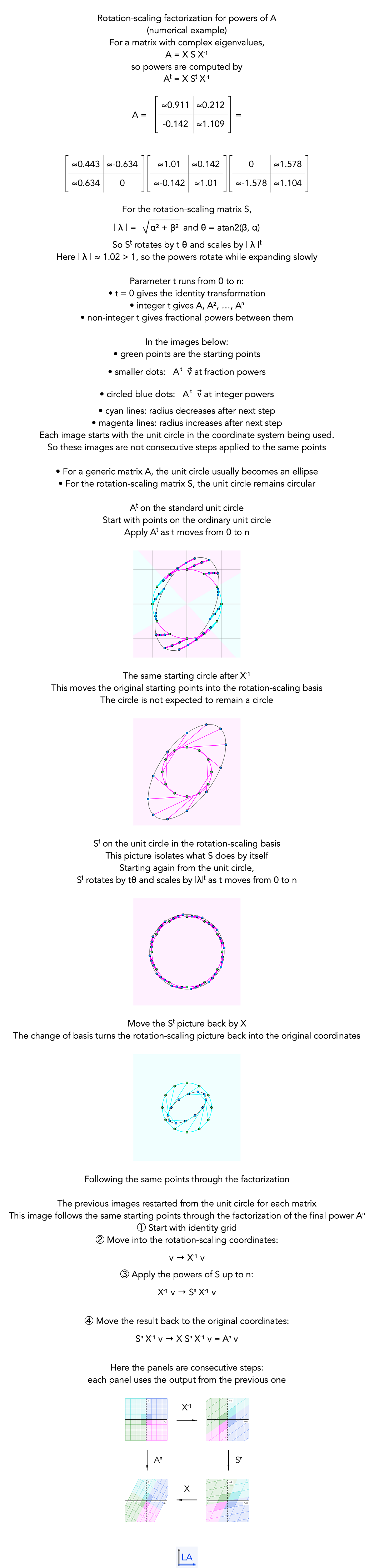
Rotation, scaling and repeated matrix powers in the complex-eigenvalue case

When a real 2D matrix has complex eigenvalues, it does not have real eigenvectors, so the usual picture of stretching along invariant real directions no longer applies. Even so, the powers of the matrix are far from mysterious. In a suitable basis, the transformation behaves like a rotation combined with scaling, and that structure controls what happens under repeated multiplication.

Explore more on GraphMath Linear Algebra

What changes in the complex-eigenvalue case?

For matrices with real eigenvectors, repeated powers are often understood through invariant lines. In the complex-eigenvalue case, there are no nonzero real vectors satisfying A x⃗ = λ x⃗ with real λ. Instead, the transformation acts like a turn together with a uniform scaling in a transformed coordinate system. That is why the geometry of A^k is naturally described by rotation, scaling and orbit behavior.

Visual guide to powers of a 2D matrix with complex eigenvalues, showing the factorization viewpoint for A to the k. — **Factorization view.** This image emphasizes that the powers of the matrix can be organized through a change of basis and a rotation-scaling core. Instead of recalculating each power independently, it shows the common internal structure behind all powers **A^k**. Click for the full-size image.

Why the factorization matters

The factorization view is useful because it separates the power computation into understandable parts:

a change of basis into coordinates where the action is simpler,
a repeated rotation by a fixed angle,
a repeated scaling by a fixed factor.

This explains why powers of such a matrix often show a clean spiral or cyclic pattern, rather than irregular behavior.

Visual guide to the orbit geometry produced by repeated powers of a real 2D matrix with complex eigenvalues. — **Orbit view.** This image focuses on what repeated powers do geometrically to vectors. Depending on the scaling factor, iterates may spiral inward, stay on a closed orbit, or spiral outward, while the rotational part keeps turning the vector at each step. Click for the full-size image.

How to read the orbit picture

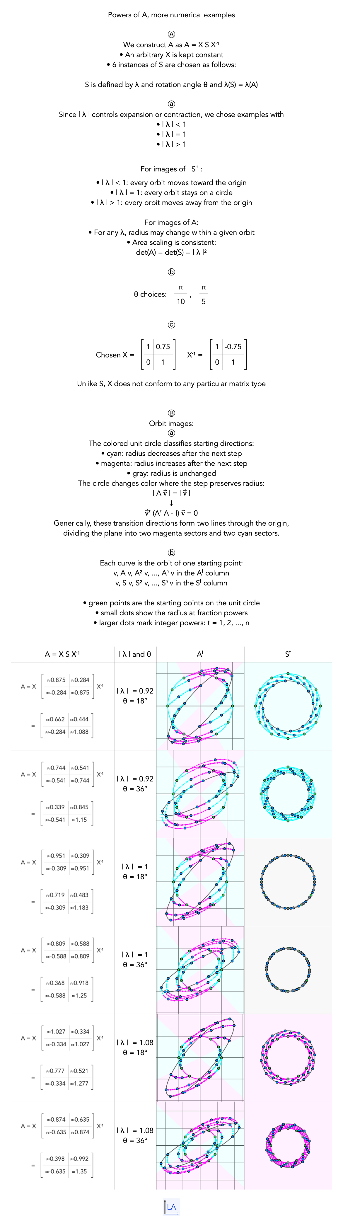
The orbit view answers a different question from the factorization view. Instead of asking how to write A^k, it asks what happens to a vector after applying the matrix again and again. This helps connect algebraic formulas with visible geometric behavior:

if the scaling factor is less than 1 in magnitude, the orbit spirals inward,
if the scaling factor has magnitude 1, the motion stays on a bounded orbit,
if the scaling factor is greater than 1 in magnitude, the orbit spirals outward.

Why these two images belong together

The first image explains the algebraic structure of matrix powers, while the second shows the geometric effect of repeated application. Together they make the complex-eigenvalue case easier to remember: even without real eigenvectors, the transformation still has a clear internal pattern, and that pattern becomes visible through rotation-scaling and orbits.

Key equations

A = X S X⁻¹

Aᵏ = X Sᵏ X⁻¹

λ = α + iβ = ρ(cos θ + i sin θ)

ρ = |λ| = √(α² + β²)

Sᵏ = ρᵏ R(kθ)

The modulus ρ controls contraction or expansion, while the angle θ controls rotation. After k applications, the scaling becomes ρ^k and the accumulated rotation becomes kθ.

Query phrases

powers of a matrix with complex eigenvalues
2D matrix powers visualization
complex eigenvalues matrix powers
rotation-scaling matrix powers
real matrix with complex eigenvalues visualization
spiral orbits from matrix powers
geometric meaning of matrix powers with complex eigenvalues
A to the k rotation scaling factorization