The Four Fundamental Subspaces

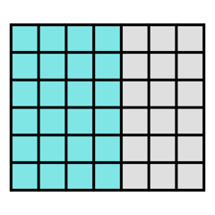
Suppose A is an (m=6)×(n=7) matrix with rank r=4
⇔
r independent columns (highlighted) & r independent rows (highlighted)
(independent rows may appear in any order)

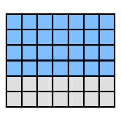
Schematic matrix A with r independent rows highlighted and remaining rows gray.

Matrix-vector product A·x⃗ is defined for all n×1 vectors x⃗

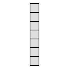
Schematic column vector x with n entries.

⊙ Domain of A is a set of all x⃗ where A·x⃗ is defined
⇔
ℝⁿ
Domain of A (or ℝⁿ) can be decomposed into two complementary subspaces:
① All linear combinations of independent rows of A, shown as an r-dimensional subspace of ℝⁿ

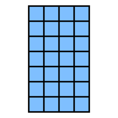
Schematic r-dimensional subspace of R^n representing the row space. — called row space of A

⇔ independent rows of A provide basis for this subspace

② Subset of all x⃗ where A·x⃗ = 0, called null space of A
(here each vector represents a direction: the whole line { c·x⃗ : c ∈ ℝ })

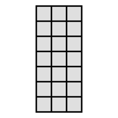
Schematic (n-r)-dimensional subspace of R^n representing the null space.

• Null space ⊕ row space = ℝⁿ (their dimensions add up to n)
⇔
every vector in ℝⁿ can be represented as (x⃗ ∈ row space) + (x⃗ ∈ null space)
⇔
they are complements of each other

• For every x⃗ in the null space, A·x⃗ = 0
↓
aᶦ · x⃗ = 0 (aᶦ are rows of A)
↓
null space is orthogonal to row space

Same matrix A is shown with independent columns highlighted:
(independent columns may appear in any order)

Schematic matrix A with r independent columns highlighted and remaining columns gray.

⊙ Codomain of A is a set of all vectors b⃗ of size m

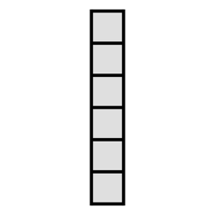
Schematic column vector b with m entries.

↓
ℝᵐ

Codomain of A (or ℝᵐ) also can be decomposed into two complementary subspaces:
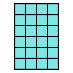
③ Range of A: subset of b⃗ that can be written as b⃗ = A·x⃗
where any b⃗ is a linear combination of columns of A with coefficients from x⃗
↓
Range of A is a linear combination of columns of A
⇔
columns of A

Schematic r-dimensional subspace of R^m representing the column space (range).

④ Left null space of A: subset of b⃗ where b⃗ᵀ·A = 0
shown as (m−r)-dimensional subspace of ℝᵐ

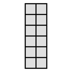
Schematic (m-r)-dimensional subspace of R^m representing the left null space.

• Column space ⊕ left null space = ℝᵐ (their dimensions add up to m)
⇔
every vector in ℝᵐ can be represented as (b⃗ ∈ column space) + (b⃗ ∈ left null space)
⇔
they are complements of each other

• For every b⃗ in the left null space, b⃗ᵀ·A = 0
↓
b⃗ᵀ · aᶦ = 0 (aᶦ are columns of A)
↓
left null space is orthogonal to column space

Summary table

Space	Lives in	Dimension	Defined as
Row space	ℝⁿ	r	Linear combinations of rows of A
Null space	ℝⁿ	n − r	Solutions of A·x⃗ = 0
Column space	ℝᵐ	r	Linear combinations of columns of A
Left null space	ℝᵐ	m − r	Solutions of b⃗ᵀ·A = 0