The four subspaces of A

1. The four subspaces of A: introduction

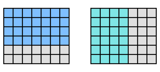
Suppose A is an (m=6)×(n=7) matrix with rank r=4

• r independent rows highlighted (left)
• r independent columns highlighted (right):
independent rows & columns may appear in any order

Matrix-vector product A×x⃗ is defined for all n×1 vectors x⃗

• Domain of A is a set of all x⃗ where A×x⃗ is defined
⇔
ℝⁿ
Domain of A or ℝⁿ can be decomposed into two complementary subspaces:
① All linear combinations of independent rows of A,
shown as an r-dimensional subspace of ℝⁿ

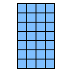
called row space of A
⇔
independent rows of A provide basis for this subspace

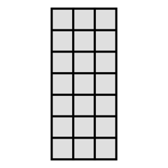
② Subset of all x⃗ where A×x⃗ = 0, called null space of A
(here each vector represents a direction: the whole line { c×x⃗ : c ∈ ℝ })

• null space ⊕ row space = ℝⁿ or the two subspaces are complements of each other
This statement means the following is true:
• their dimensions add up to n
• they do not overlap or, equivalently, the only intersection is zero vector
• every vector x⃗ in ℝⁿ has a unique representation as (x⃗∥ ∈ row space) + (x⃗⊥ ∈ null space)

• Note that for every x⃗ in the null space, A×x⃗ = 0
⇩
aⁱ · x⃗ = 0 (aⁱ are rows of A)
⇩
every vector in null space is orthogonal to every vector in row space

• Codomain of A is a set of all vectors b⃗ of size m

⇩
ℝᵐ
Codomain of A or ℝᵐ also can be decomposed into two complementary subspaces:
③ Range (column space) of A: subset of b⃗ that can be written as b⃗ = A×x⃗
where any b⃗ is a linear combination of columns of A with coefficients from x⃗
⇩
Range of A is a linear combination of columns of A
⇔
columns of A provide basis for this subspace

④ Left null space of A: subset of b⃗ where b⃗ᵀ×A = 0
shown as (m-r)-dimensional subspace of ℝᵐ

• column space ⊕ left null space = ℝᵐ or the two subspaces are complements of each other
This statement means the following is true:
• their dimensions add up to m (r + (m-r) = m)
• they do not overlap or, equivalently, the only intersection is zero vector
• every vector b⃗ in ℝᵐ has a unique representation as (b⃗∥ ∈ column space) + (b⃗⊥ ∈ left null space)

• Note that for every b⃗ in the left null space, b⃗ᵀ×A = 0
⇩
b⃗ᵀ · aⁱ = 0 (aⁱ are columns of A)
⇩
every vector in left null space is orthogonal to every vector in column space

---

2. Definitions

① Vector space 𝒱 or ℝⁿ:
collection of all vectors with n components
Example: ℝ³

② Subspace 𝒮 of 𝒱:
collection of all vectors satisfying following:
• for any vectors x⃗ & y⃗ inside 𝒮, all of their linear combinations are also inside 𝒮
(which also implies that 𝒮 includes the zero vector)
Examples: plane, line or zero vector in ℝ³ (through the origin)

③ Complementary subspaces 𝒮1 & 𝒮2 of 𝒱 satisfy following conditions:
• intersect only at 0
• every vector x⃗ in 𝒱 can be written uniquely as x⃗ = x⃗1 + x⃗2 with x⃗1 in 𝒮1 and x⃗2 in 𝒮2
or, equivalently, 𝒮1 & 𝒮2 span 𝒱

④ Orthogonal subspaces 𝒮1 & 𝒮2 satisfy following condition:
every vector in 𝒮1 is orthogonal to every vector in 𝒮2

Note:
• Complementary does not imply orthogonal
• Orthogonal does not imply complementary (𝒮1 & 𝒮2 may not span 𝒱)
• 𝒮2 as the set of ALL vectors orthogonal to all vectors in 𝒮1
does imply complementary (𝒮1 & 𝒮2 span 𝒱)
• If 𝒮1 & 𝒮2 are complementary,
most vectors do not lie entirely in 𝒮1 or 𝒮2:
they have components in both 𝒮1 & 𝒮2
• Complementary is a dimension condition:
dim(𝒮1) + dim(𝒮2) = dim(𝒱) and 𝒮1 ∩ 𝒮2 = {0}

---

3. Geometric interpretation of the four subspaces of A

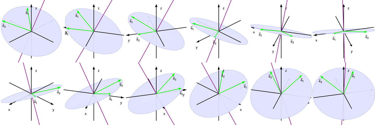
Suppose we have a 3×2 matrix A = [ a⃗₁ | a⃗₂ ]
where a⃗₁ & a⃗₂ are linearly independent vectors in ℝ³,
so rank(A) = 2

① Domain(A) = ℝ², an abstract 2D coefficient space, or an abstract plane

② null space(A) or all directions in the domain (ℝ²) that produce 0⃗ output:
For the given A, only the 0⃗ vector:
• Dimension: n-r=0 in ℝ²
• Every vector from the domain produces a unique output
⇔
Transformation is one-to-one

③ row space(A)
While rows of A cannot be directly visualized in the same image as columns,
row space is a set of all vectors in the domain that are orthogonal to null space,
or, equivalently,
set of all vectors that have 0 component in the null space
For the given A, all vectors in ℝ² satisfy the condition
• Dimension: r=2 in ℝ²

④ Codomain(A) is a set of all vectors in ℝ³

⑤ column space(A) or all linear combinations of a⃗₁ & a⃗₂
or the plane spanned by the two vectors
in ℝ³ and expressed in 3D coordinates
• Dimension: r=2 in ℝ³
• Output does not fill the codomain
⇔
Transformation is not onto

⑥ ℓ-null space(A) or all directions in the codomain (ℝ³) orthogonal to column space:
all vectors along the orthogonal line, shown in purple
• Dimension: m-r=1 in ℝ³

⑦ Matrix A
• takes a set of all vectors in ℝ² and transforms them in a way that
• (1, 0) maps to a⃗₁
• (0, 1) maps to a⃗₂
• all other vectors x⃗ follow as x₁a⃗₁ + x₂a⃗₂, which fills the blue plane in ℝ³

⑧ Matrix Aᵀ
• takes vectors in ℝ³ and transforms them in a way that
• a⃗₁ maps to AᵀA column 1
• a⃗₂ maps to AᵀA column 2
• all other 3D vectors y⃗ 'follow suit' and are now expressed in 2D coordinates

⑨ Matrix AᵀA acts entirely inside ℝ² in a way that
• (1, 0) maps to AᵀA column 1
• (0, 1) maps to AᵀA column 2

---

4. The four subspaces of A: summary table

• Domain (ℝⁿ) = row space ⊕ null space

• Codomain (ℝᵐ) = column space ⊕ ℓ-null space

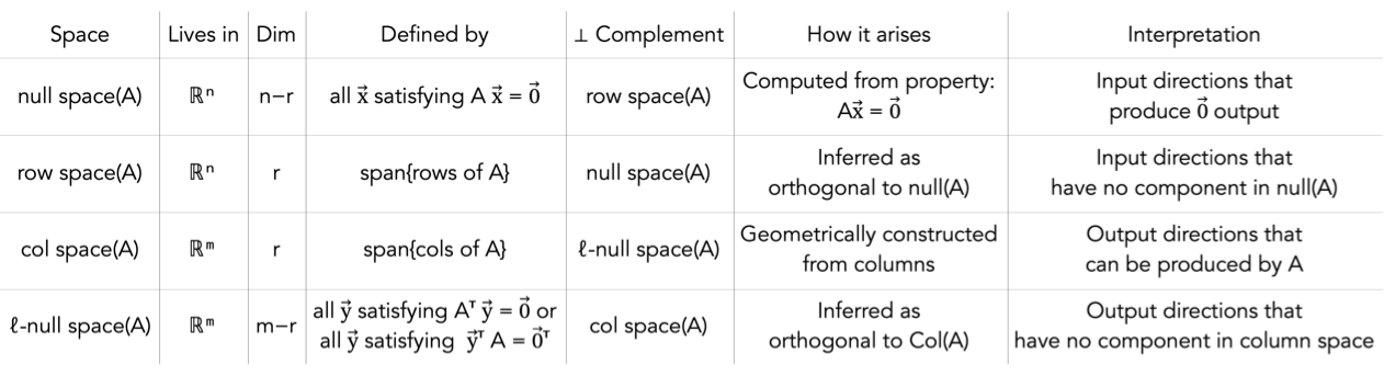
Note how the 'deduced' space orthogonal to null(A) becomes row space: suppose
• B = Aᵀ and Bᵀ = A
• row space(A) = col space (B) & col space (B) = row space(A)
• vector y⃗ satisfying y⃗ᵀ B = 0⃗ᵀ is in the ℓ-null space (B)
• same vector y⃗ also satisfies Bᵀ y⃗ = 0⃗, same as A y⃗ = 0⃗
• same vector y⃗ belongs to null space (A)
• orthogonal complement of ℓ-null space (B) is column space (B), same as row space(A)
⇩
The set of all vectors orthogonal to null space(A) is precisely the row space(A)

We propose starting with the two primary spaces:
1. column space(A) in ℝᵐ (what A can produce, can be visualized directly)
2. null space(A) in ℝⁿ (solutions to Ax⃗ = 0, can be computed directly)

The remaining two subspaces are inferred as orthogonal complements to the primary ones